Thursday, May 12, 2016
Final Report
Please check out our final report documenting our work and results!
ESE 350 - Tunable Analog Hearing Aid - Final Report
ESE 350 - Tunable Analog Hearing Aid - Final Report
Thursday, April 28, 2016
Test results
We ran some test using resistor values from the optimiser and got several frequency response charts from it.
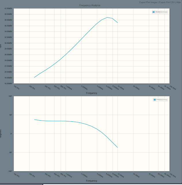
 This is the result through a single filter. The yellow is the input and the blue is the output. The size is expected because we use the summing amplifer to do most of the amplification. In addition we were expecting the output to grow at higher frequencies given the input to the optimizer.
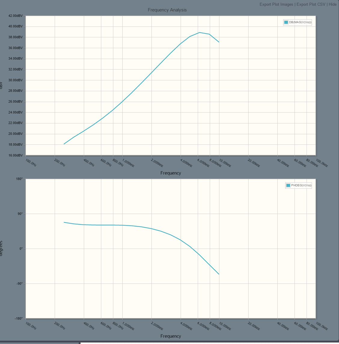
 This is the result through the pass-through filter. This as well is what we expected - simple reduction is amplitude so when it goes through the summing amplifier it is the correct magnitude.

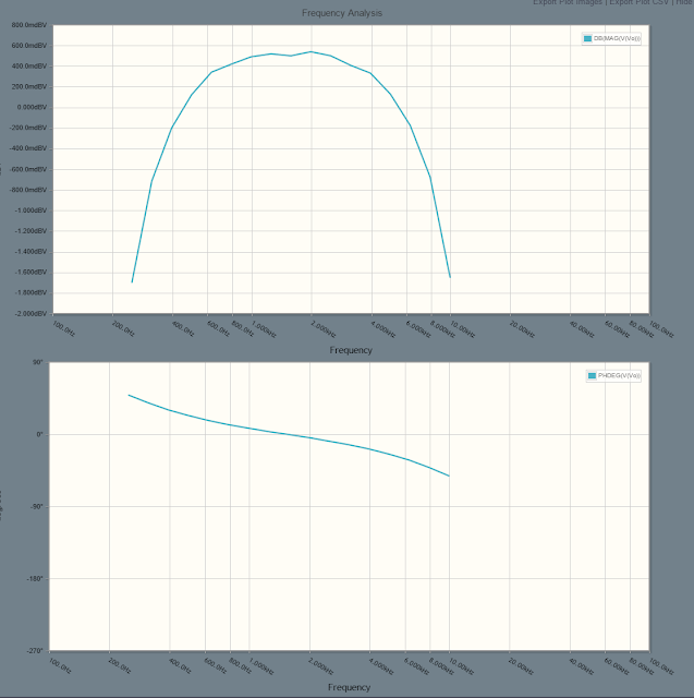
 We can see that the phase is -90 degrees for most of the bandwidth and then gets worse as we near the peak. When two waves are 180 degress out of phase, they cancel perfectly. This is clearly a problem we did not anticipate and are not accounting for in the optimization. We are currently looking into solutions involving phase shift circuitry or different ways of optimizing the values.


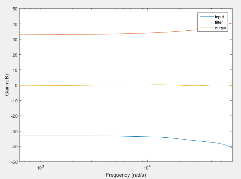
This is where things get interesting. This is the final outpu from the summing amplifer. We would expect this to be a simple sum of the two magnitudes. However, unlike the first output, it is actually smaller at higher frequencies.
We currently think that the problem has to do with phase. If we look at the phase of the bandpass filters we are using:

Implementation
For implementation we decided to start small with only two bandpass filters. This is easy because we are using LM358 opamp chips which each have two op-amps per chip. Each filter requires 3 resistors as well as a gain potentiometer. For this reason, we got MCP4261 chips. These are variable potentiometers with two potentiometers per IC. This lets us create a full filter with only two resistor chips and half of an op-amp chip. We also decided to add the unmodified input to the summing amplifier. This lets us set a gain across the spectrum in the case that the user has general hearing loss across all frequencies.

In the center, there are five ICs. Four of them are the MCP4261. Under the crossed yellow wires is the LM358 chip. These five ICs make up the two bandpass filters we have so far. Beneath them on the same column is another MCP4261, this chip is used to set the gain on the pass-through data. On the bottom left, there is a summing amplifer that takes the three voltages from the filters and pass-through and creates a final output.
On the left is an mbed. We use this to program the MCP4261s over SPI.
MATLAB Optimization Results
Before testing our MATLAB optimization on audiograms, we validated the individual parts of the algorithm, including the bandpass filter function we created and the method of combining frequency response graphs against circuit simulations in CircuitLab. After this validation process, we tested the entire script on audiogram samples.
Figure 4 above is a low pass filter representation of a hearing impaired person's audiogram. This result will be used for testing and validation of the optimization in our circuit.
The following figures show the optimization script's ability to compensate for various types of hearing loss, including sensineural, conductive, and mixed. In all of these cases, the algorithm performs well and is able to bring the output hearing to a normal range of -20 dB - 10. However, for the mixed hearing loss, there is a small dip below -20 dB at roughly 15000 rad/s. This indicates that we may need an additional bandpass filter in the higher frequency regions or higher gain capabilities.
 |
| Figure 1: Sensineural Audiogram |
 |
| Figure 2: Conducitve Audiogram |
 |
| Figure 3: Mixed Audiogram |
 |
| Figure 4: Low Pass filter representation of audiogram |
Wednesday, April 27, 2016
Prototype 1 - Functional Block Diagrams
We have completed prototype 1. This prototype consists of a circuit containing 2 programmable bandpass filters and programmable gains for each filter and the original sound wave. A final programmable gain is also included. The functional block diagram is shown in Figure 1. Details of the implementation of this circuit will be posted soon.
In order to determine the optimal filter and gain values for the circuit in Figure 1, we created a MATLAB script that performed frequency response analysis of our circuit and utilized a non linear least squared optimizer. A functional block diagram of the optimization script is shown in Figure 2.
The cost function used for the non linear optimization combines the frequency response magnitude curves of each of the parallel band pass filters and the original sound signal. The optimal function y = 0 represents an ideal frequency response, which is a decibel gain of 0. This signifies no deviation in amplitude from the original sound.
The non linear optimization function, in this case the MATLAB function lsqnonlin, attempts to minimize the difference between the ideal function and the filter circuit by varying the desired parameters of the filter resistors and gains. The function then outputs the variables found by the optimization.
The band pass filters were modeled using the following transfer function model for an MFB bandpass filter:


 Each resistor value, R1, R2, and R3, was varied during the optimization.
 |
| Figure 1: Functional Block Diagram of circuit for prototype 1 |
In order to determine the optimal filter and gain values for the circuit in Figure 1, we created a MATLAB script that performed frequency response analysis of our circuit and utilized a non linear least squared optimizer. A functional block diagram of the optimization script is shown in Figure 2.
 |
| Figure 2: Functional Block Diagram |
The cost function used for the non linear optimization combines the frequency response magnitude curves of each of the parallel band pass filters and the original sound signal. The optimal function y = 0 represents an ideal frequency response, which is a decibel gain of 0. This signifies no deviation in amplitude from the original sound.
The non linear optimization function, in this case the MATLAB function lsqnonlin, attempts to minimize the difference between the ideal function and the filter circuit by varying the desired parameters of the filter resistors and gains. The function then outputs the variables found by the optimization.
The band pass filters were modeled using the following transfer function model for an MFB bandpass filter:


Friday, April 15, 2016
We ran several simulations of filter designs during prototyping. We very quickly came to the general idea of using several bandpass filters to handle various bands of frequency separately and then combine the outputs together using a summing amplifier. It took us another week to settle on the filter design and parameters as well as the number of filters. We eventually settled on 6 1st order bandpass filters with center frequencies evenly spaced out between 250Hz and 10000Hz. This gave us the following design.


If we modify the resistor values of each filter we have total control over center frequency, gain and quality factor, though the "standard" values shown give a smooth, neutral amplification:

If the user needs amplification at high frequencies we can modify the gain resistors to get the following response:
We also studied the possibility of chaining the filters by passing the output of one to the input of another. This would give us a higher roll-off rate and could be used by adding some switching circuitry. The use case of this would be a user with a significant amount of hearing loss in certain bandwidths and no hearing loss in others. In this case, we would not want to overamplify the bandwidth in which their hearing is not impaired.
An example response is like this:

Here, the roll-off rate is twice that of the previous filter and has useful amplification only in the requested areas.
Subscribe to:
Posts (Atom)